Eigenvalues and eigenvectors - physical meaning and geometric interpretation applet
Introduction
We learned in the previous section, Matrices and Linear Transformations that we can achieve reflection, rotation, scaling, skewing and translation of a point (or set of points) using matrix multiplication. We were transforming a vector of points v into another set of points vR by multiplying by some square matrix A as follows:
Av = vR
In the following sections, we will learn how to find eigenvalues and eigenvectors of a matrix, but before we do, let's see what those words mean.
Our aim is to replace our square matrix A with some scalar (number) λ for a particular vector v so we'll have:
Av = λv = vR
The scalar λ is called an eigenvalue, and v is called the corresponding eigenvector of A.
(The German word "eigen" roughly translates as "own" or "belonging to".)
The interactive
The following applet begins to answer the question "What are eigenvalues and eigenvectors?"
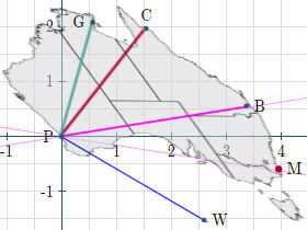
Scenario: Various aircraft fly to and from Perth, placed at P(0, 0) on the map below, to different parts of Australia. The cities involved are:
- Brisbane, at B(3.8, 0.6), the capital of Queensland state.
- Cairns, at C(3, 2), near the Great barrier Reef.
- Gove, at G(2.1, 2.1), directly NE of Perth, in the remote Northern Territory.
- An oil well at W(1, −1), due SE of Perth, in the Great Australian Bight.
We'll distort the map to demonstrate what is meant by eigenvalues and eigenvectors.
Things to do
After reading the description, move the slider (labelled "skewB") to distort the map in a particular way. What we'll see is the eigenvalue and corresponding eigenvector relating to the journey Perth to Brisbane.
Then, follow the instructions given to move on to the other examples.
Disclaimer: We are only attempting to illustrate cases where each of matrices A, v are real and the scalar λ is real too. For cases where complex numbers are involved, this "squashed map" illustration does not hold.
The explanation updates as you change the sliders.
Copyright © www.intmath.com
Summary of the applet
skewB: Eigenvectors at Brisbane and M

Points along the line PB remain at the same slope as we change matrix A. Here's a typical value.
`bb(Av)=[(1,-0.5),(-0.01,1)][(3.8),(0.6)]`
`= [(3.5),(0.55)]`
`= 0.9211[(3.8),(0.6)]`
`=lambda bb(v)`
We've replaced matrix A with a scalar value λ, but only along the line PB.
We can do the same along line PM, since any point M on that line represents the other eigenvector, and the scale of the distance PM represents the corresponding eigenvalue for vector M.
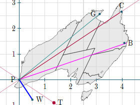
skewC: Eigenvectors at Cairns and T

Points along the line PB remain at the same slope as we change matrix A. Here's a typical value.
`bb(Av)=[(1,0.5),(0.22,1)][(3),(2)]`
`= [(4),(2.67)]`
`= 1.3333[(3),(2)]`
`=lambda bb(v)`
We've replaced matrix A with a scalar value λ, but only along the line PB.
We can do the same along line PM, since any point M on that line represents the other eigenvector, and the scale of the distance PM represents the corresponding eigenvalue for vector M.
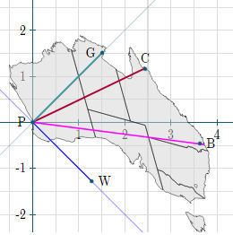
skewXY: Eigenvectors at Gove and W

Points along the line PG remain at the same slope as we change matrix A. Here's a typical value.
`bb(Av)=[(1,-0.29),(-0.29,1)][(2.1),(2.1)]`
`= [(1.5),(1.5)]`
`= 0.7143[(2.1),(2.1)]`
`=lambda bb(v)`
We've replaced matrix A with a scalar value λ, but only along the line PG.
We can do the same along line PW, since any point W on that line represents the other eigenvector, and the scale of the distance PW represents the corresponding eigenvalue for vector W.
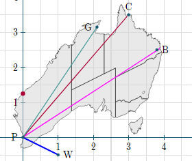
skewXorY: Eigenvectors along the axes only

The only directions that remain at the same slope as we change matrix A are along either the x- or y- axes. Here's a typical value, for the "skewY" case:
`bb(Av)=[(1,0),(0.5,1)][(3),(2)]`
`= [(3),(3.5)]`
This time, we haven't been able to replace the matrix A with a scalar value. There is a double eigenvalue of 1 and the eigenvectors are in the direction of the x- or y- axes.
Further information
a. Why do we need eigenvalues and eigenvectors?
Many "real world" matrices have thousands of rows and columns, which take up a lot of computing power. If we can reduce (or approximate) those large matrices to a single number, it speeds things up considerably.
See Applications of Eigenvalues and Eigenvectors for some of the ways eigenvalues and eigenvectors are used.
b. Where did those matrices causing a skew transform come from?
For the "skewB" case in the applet, the matrix used was based on the following:
`bb(A_1)=[(1,-s^2 tan(theta)), (-tan(theta),1)]`
where
s is the slope of the line PB, in this case `s=0.6/3.8= 0.15789`, giving `s^2=0.02493,` and
θ is the skew angle.
For the "skewC" case, the matrix had the same form, with `s=2/3`, giving `s^2=0.44444.`
For the "skewXY" case, the slope is `1`, so `s^2=1.`
c. What are the second eigenvalues and eigenvectors in each case?
For "skewB", the point M is (3.55, −0.55), (the slope of line PM is the negative of the line PB) with eigenvalue λ2 = 1, our eigenvector will be `bb(v)_2=[(3.55),(-0.55)].`
For "skewC", the point T is (2.5, −1.67), (once again, the reflection in the x-axis) so with eigenvalue λ4 = 1, our eigenvector will be `bb(v)_4=[(2.5),(-1.67)].`
For "skewXY", the point W is (1.5, −1.5), (the reflection in the x-axis of the PG vector) so with eigenvalue λ6 = 1, our eigenvector will be `bb(v)_6=[(1.5),(-1.5)].`
Math used in the above applet
Here is some of the math used to create the above applet.
- Multiplying matrices
- Skewing a shape
- Converting angles in radians (which javascript requires) to degrees (which is easier for humans) and vice-versa
- Absolute value (for formatting negative numbers)
- Inequalities (many "if" clauses and animations involve inequalities)
Credit: Australia map (Wikipedia)
Next, we'll see how to Find eigenvectors and eigenvalues for a square matrix ».